Capacitor & Capacitance: Extra Knowledge !

Capacitance of simple systems

Calculating the capacitance of a system amounts to solving the Laplace equation ∇²φ=0 with a constant potential φ on the surface of the conductors. This is trivial in cases with high symmetry. There is no solution in terms of elementary functions in more complicated cases.

For quasi-two-dimensional situations analytic functions may be used to map different geometries to each other. See also Schwarz-Christoffel mapping.

Capacitance of simple systems
Type	Capacitance	Comment
Parallel-plate capacitor	$\varepsilon A /d$	ε: Permittivity
Coaxial cable	$\frac{2\pi \varepsilon l}{\ln \left( R_{2}/R_{1}\right) }$	ε: Permittivity
Pair of parallel wires	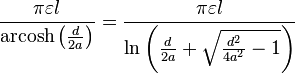$\frac{\pi \varepsilon l}{\operatorname{arcosh}\left( \frac{d}{2a}\right) }=\frac{\pi \varepsilon l}{\ln \left( \frac{d}{2a}+\sqrt{\frac{d^{2}}{4a^{2}}-1}\right) }$
Wire parallel to wall	$\frac{2\pi \varepsilon l}{\operatorname{arcosh}\left( \frac{d}{a}\right) }=\frac{2\pi \varepsilon l}{\ln \left( \frac{d}{a}+\sqrt{\frac{d^{2}}{a^{2}}-1}\right) }$	a: Wire radius d: Distance, d > a $l$ : Wire length
Two parallel coplanar strips	$\varepsilon l \frac{ K\left( \sqrt{1-k^{2}} \right) }{ K\left(k \right) }$	d: Distance w₁, w₂: Strip width k_i: d/(2w_i+d) k²: k₁k₂ K: Elliptic integral $l$ : Length
Concentric spheres	$\frac{4\pi \varepsilon}{\frac{1}{R_{1}}-\frac{1}{R_{2}}}$	ε: Permittivity
Two spheres, equal radius	$2\pi \varepsilon a\sum_{n=1}^{\infty }\frac{\sinh \left( \ln \left( D+\sqrt{D^{2}-1}\right) \right) }{\sinh \left( n\ln \left( D+\sqrt{ D^{2}-1}\right) \right) }$ $=2\pi \varepsilon a\left\{ 1+\frac{1}{2D}+\frac{1}{4D^{2}}+\frac{1}{8D^{3}}+\frac{1}{8D^{4}}+\frac{3}{32D^{5}}+O\left( \frac{1}{D^{6}}\right) \right\}$ $=2\pi \varepsilon a\left\{ \ln 2+\gamma -\frac{1}{2}\ln \left( \frac{d}{a}-2\right) +O\left( \frac{d}{a}-2\right) \right\}$	a: Radius d: Distance, d > 2a D = d/2a γ: Euler's constant
Sphere in front of wall	$4\pi \varepsilon a\sum_{n=1}^{\infty }\frac{\sinh \left( \ln \left( D+\sqrt{D^{2}-1}\right) \right) }{\sinh \left( n\ln \left( D+\sqrt{ D^{2}-1}\right) \right) }$	a: Radius d: Distance, d > a D = d/a
Sphere	$4\pi \varepsilon a$	a: Radius
Circular disc	$8\varepsilon a$	a: Radius
Thin straight wire, finite length	$\frac{2\pi \varepsilon l}{\Lambda }\left\{ 1+\frac{1}{\Lambda }\left( 1-\ln 2\right) +\frac{1}{\Lambda ^{2}}\left[ 1+\left( 1-\ln 2\right) ^{2}-\frac{\pi ^{2}}{12}\right] +O\left(\frac{1}{\Lambda ^{3}}\right) \right\}$	a: Wire radius $l$ : Length Λ: ln( $l$ /a)

Wednesday, 19 December 2012

Extra Knowledge !

Capacitance of simple systems

No comments:

Post a Comment